 Graziano & Raulin
Research Methods (9th edition)
Comparing Two Independent Samples
In the previous section, you were introduced the the logic of the t-test. You learned that you could test whether the mean from a single group of subjects came from a hypothetical population with a specified mean. The logic involved recognizing that:
- The means drawn from such a population would be distributed as a t distribution, which is a symmetric distribution that is a bit flatter than the standard normal distribution, but very close to the standard normal distribution when the sample size is large.
- The critical value of t can be looked up in a table if you specify the alpha level and whether you want to conduct a one-tail or two-tail test and if you know the degrees of freedom. For the single-group t-test, the degrees of freedom are equal to N minus 1.
- The t is computed by using a formula that includes the sample mean and standard deviation, the sample size, and the hypothesized population mean. If the size of the computed t exceeds the critical value of t, you reject the null hypothesis that the sample came from a population with that specified sample mean.
The logic specified here boils down to this: The single-group t-test essentially determines whether the sample mean would fall in the hypothetical distribution of means for samples of the size specified from the hypothetical population specified. We can create this distribution because we know its shape (the t distribution), it mean (the population mean that we specified), and its standard deviation (the standard error of the mean, which is a function of the standard deviation of the population and the samples size). We are able to estimate the standard deviation of the population using our standard deviation from our sample (Note that we use the unbiased estimate of the standard deviation).
We are now going to take this same logic and extend it to a situation that you will encounter much more frequently in psychological research. The situation is the comparison of two groups of participants. These might be two existing groups, such as males and females, which represents differential research (see Chapter 7 of the text). Alternatively, these might be two randomly assigned groups that experience different treatments, which represents experimental research (see Chapter 10 of the text).
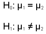
Whatever the case, we are going to compare these two groups using the same logic outlined for the one group situation. The null hypothesis will be that the population means for the two groups are equal, and the nondirectional alternative hypothesis will be that they are not equal (this if for the two-tail test). These hypotheses are specified below, with the subscripts 1 and 2 representing the two groups.
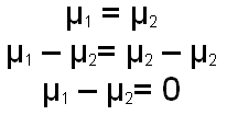
The difference here is that we are no longer looking at the sampling distribution of means, but rather are looking at the sampling distribution of the difference between the two means. We know that if the null hypothesis is true (the population means are equal), the the mean of the difference between the two means should be zero. We can can prove this with some very straight forward algebra, as shown below.
We also know what the standard deviation of the distribution of means would be. The formula for computing it from the population standard deviations is given below. Of course, we don't know the population standard deviations, but we can estimate them with the sample standard deviations. The second formula shows how we would estimate, using the sample standard deviations and the sample sizes, the standard deviation of the distribution of the difference between the two means.
That last phrase is quite a mouthful. This standard deviation is referred to as the standard error of the mean difference or more commonly is shortened to standard error. If you use the shorter notation of standard error, you must remember that there are different standard errors for different statistical tests, so you must keep the formulas straight.
The algebra for how this formula estimates the variability of this distribution of mean differences is a lot more complicated, so you are better off taking our word that this formula is correct. Finally, we know that the shape of the distribution of mean differences will be a t distribution, with the degrees of freedom equal to the sum of the two sample sizes minus 2 (i.e., df=N1+N2-2). Again, showing why this is the case is well beyond the level of this text, so take our word for it. However, it all comes together with the two-sample t-test, often called the simple t-test or just the t-test.
The formulas for this test are shown below.
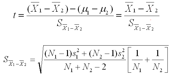
These equations are certainly more complicated than any you have seen so far in this statistical concepts section, but they are not as complicated as they seem. Let's start by looking at the first equation. It says that we will be taking the mean difference of the samples, subtracting the mean difference of the populations, and dividing by the Standard error of that mean difference. If you go back to the single-group t-test, you will see that this is exactly parallel. There we took the sample mean, subtracted the population mean, and divided by the standard error of the mean.
The second part of the first equation eliminated the population mean difference, because under the null hypothesis (of no difference), that mean difference is zero. The second equation looks more complex than it is, and we skipped over how it was derived. You really do not need to know how it was derived to understand the principle here. This equation gives you the standard error of the mean difference. As complicated as it looks, there are only 4 variables in the equation (the variance for each group and the sample size for each group). In both of these equations, the subscripts of 1 and 2 are for the two groups being evaluated.
You can see examples of how a t-test for two groups is computed either manually or using SPSS for Windows by clicking on one of the links below. Use the back arrow key to return to this page when you are done. Although tedious, this computation can be done manually, but it is certainly easier to rely on a computer to do the analysis.
|
Compute the t-test for independent groups by hand |
|
Compute the t-test for independent groups using SPSS |
|
USE THE BROWSER'S |
Note that this procedure is for the situation in which you are evaluating two independent groups, which means that there are different people in each group and there is no matching of individuals in the groups (see Chapter 10 in the text).
The next section of the statistical concepts unit will introduce you to the procedure for analyzing the difference between two correlated groups (see Chapter 11 of the text).