 Graziano & Raulin
Research Methods (9th edition)
Computational Procedures for a
Repeated-Measures ANOVA
The Raw Data
In this example, we will compute a repeated-measures ANOVA for data from six participants tested under three conditions. The raw data for the 6 participants, tested under three conditions, are listed below. Please note that it is assumed that appropriate controls for sequence effects were used (e.g., counterbalancing). Nevertheless, we arrange the data in columns by condition, as shown below, regardless of what order the participant received the conditions. We have also included a fourth column in which we summed the scores across the three conditions. These totals will be used in later computations.
| Participant | Condition 1 | Condition 2 | Condition 3 | Sum Total |
| A | 10 | 8 | 8 | 26 |
| B | 12 | 9 | 8 | 29 |
| C | 11 | 10 | 9 | 30 |
| D | 11 | 10 | 8 | 29 |
| E | 10 | 8 | 9 | 27 |
| F | 11 | 9 | 7 | 27 |
Summary Statistics
The first step in the computation of a repeated-measures ANOVA is to sum each column and to compute the sum of the squared scores and mean for each column. These values are shown in the matrix below. Again, we have included a fourth column in which we have summed across to get the total sum of X and the total sum of X2.
| Condition 1 | Condition 2 | Condition 3 | Sum Totals | |
| Sum of X | 65 | 54 | 49 | 168 |
| Sum of X2 | 707 | 490 | 403 | 1600 |
| Mean | 10.83 | 9.00 | 8.17 |
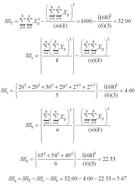
Compute the Sums of Squares (SS) for the ANOVA
We will compute three sums of squares: subjects, between, and error. Essentially, we are taking the SSw and breaking it into a subjects and an error term. What we are doing is removing the individual differences component (SSs) from what is normally the error term. The result is that our error term for this ANOVA will be smaller, and therefore this statistical procedure will be more powerful.
Again, the notation gets a bit more complicated. We use n to indicate the number of participants and k to indicate the number of conditions. When we are summing across conditions, we use summation notation that says that j goes from 1 to k. That is what we did in the raw data matrix above, when we added the scores for the three conditions for each person. When we are summing across participants, we use summation notation that say that i goes from 1 to n. Each X value has two subscripts (i and j) to indicate which participant and which condition is being referenced, respectively.
Fill in the Summary Table
The dfb is equal to the number of conditions minus 1. The dfs is equal to the total number of participants minus 1. The dfe is equal to the product of the dfb and the dfs. The dfT is equal to the number of conditions (k) times the number of participants (n), with 1 subtracted from that product (nk - 1).
Each of the MS is computed by dividing the SS by its respective df, and the F is computed by dividing the MSb by the MSe.
| Source | df | SS | MS | F |
| Between | 2 | 22.33 | 11.17 | 19.71 |
| Subjects | 5 | 4.00 | 0.80 | |
| Error | 10 | 5.67 | 0.567 | |
| Total | 17 | 32.00 |
The final step is to compare the value of the F computed in this analysis with the critical value of F in the F Table. You look up the critical value by using the degrees of freedom. In our case, the dfb is 2 and the dferror is 10. The critical value of F for an alpha of .05 is 4.10. Because our obtained F exceeds this value, we reject the null hypothesis and conclude that there is a significant difference between the conditions.